Understanding Cells
Every worksheet is made up of thousands of rectangles, which are called cells. A cell is the intersection of a row and a column. Columns are identified by letters (A, B, C), while rows are identified by numbers (1, 2,3).

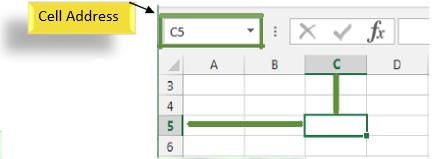
Each cell has its own name, or cell address, based on its column and row. In this example, the selected cell intersects column C and row 5, so the cell address is C5. The cell address will also appear in the Name box. Note that a cell's column and row headings are highlighted when the cell is selected.
You can also select multiple cells at the same time. A group of cells is known as a cell range. Rather than a single cell address, you will refer to a cell range using the cell addresses of the first and last cells in the cell range, separated by a colon. For example, a cell range that included cells A1, A2, A3, A4, and A5 would be written as A1:A5.
In the images below, two different cell ranges are selected:
- Cell range A1:A8

- Cell range A1:B8

To select a cell range
Sometimes you may want to select a larger group of cells, or a cell range.
- Click, hold, and drag the mouse until all of the adjoining cells you wish to select are highlighted.
- Release the mouse to select the desired cell range. The cells will remain selected until you click another cell in the worksheet.
3.2. Cell Content
Any information you enter into a spreadsheet will be stored in a cell. Each cell can contain several different kinds of content, including text, formatting, formulas, and functions.
- Text
Cells can contain text, such as letters, numbers, and dates.

- Formatting Attributes
Cells can contain formatting attributes that change the way letters, numbers, and dates are displayed. For example, percentages can appear as 0.15 or 15%. You can even change a cell's background color.
- Formulas and Functions
Cells can contain formulas and functions that calculate cell values. In our example, SUM(B4:B7) adds the value of each cell in cell range B4:B7 and displays the total in cell B8.

To insert content
- Click a cell to select it.

- Type content into the selected cell, then press Enter on your keyboard. The content will appear in the cell and the formula bar. You can also input and edit cell content in the formula bar.


To delete cell content
- Select the cell with content you wish to delete.
- Press the Delete or Backspace key on your keyboard. The cell's contents will be deleted.
To delete cells
There is an important difference between deleting the content of a cell and deleting the cell itself. If you delete the entire cell, the cells below it will shift up and replace the deleted cells.
- Select the cell(s) you wish to delete.
- Select the Delete command from the Home tab on the Ribbon.
- The cells below will shift up.

To copy and paste cell content
Excel allows you to copy content that is already entered into your spreadsheet and paste that content to other cells, which can save you time and effort.
- Select the cell(s) you wish to copy.
- Click the Copy command on the Home tab, or press Ctrl+C on your keyboard.

- Select the cell(s) where you wish to paste the content. The copied cells will now have a dashedbox around them.
- Click the Paste command on the Home tab, or press Ctrl+V on your keyboard.
- The content will be pasted into the selected cells.
To access more paste options
You can also access additional paste options, which are especially convenient when working with cells that contain formulas or formatting.
- To access more paste options, click the drop-down arrow on the Paste.

- TIP: Rather than choosing commands from the Ribbon, you can access commands quickly by right-clicking. Simply select the cell(s) you wish to format, then right-click the mouse. A drop-down menu will appear, where you'll find several commands that are also located on the Ribbon.


To drag and drop cells
Rather than cutting, copying, and pasting, you can drag and drop cells to move their contents.
- Select the cell(s) you wish to move.
- Hover the mouse over the border of the selected cell(s) until the cursor changes from a whitecross to a black cross with four arrows.
- Click, hold, and drag the cells to the desired location.
- Release the mouse, and the cells will be dropped in the selected location.
To use the fill handle
There may be times when you need to copy the content of one cell to several other cells in your worksheet. You could copy and paste the content into each cell, but this method would be very time consuming. Instead, you can use the fill handle to quickly copy and paste content to adjacent cells in the same row or column.
- Select the cell(s) containing the content you wish to use. The fill handle will appear as a small square in the bottom-right corner of the selected cell(s).

- Click, hold, and drag the fill handle until all of the cells you wish to fill are selected.

- Release the mouse to fill the selected cells.
To continue a series with the fill handle
The fill handle can also be used to continue a series. Whenever the content of a row or column follows a sequential order, like numbers (1, 2, 3) or days (Monday, Tuesday, Wednesday), the fill handle can guess what should come next in the series. In many cases, you may need to select multiple cells before using the fill handle to help Excel determine the series order. In our example below, the fill handle is used to extend a series of dates in a column.

3.3. Find and Replace
When working with a lot of data in Excel, it can be difficult and time consuming to locate specific information. You can easily search your workbook using the Find feature, which also allows you to modify content using the Replace feature.
To find content
- From the Home tab, click the Find and Select command, then select .. from the drop-down menu.

- The Find and Replace dialog box will appear. Enter the content you wish to find.
- Click Find Next. If the content is found, the cell containing that content will be selected.

- Click Find Next to find further instances or Find All to see every instance of the search term.
- When you are finished, click Close to exit the Find and Replace dialog box.
- TIP: You can also access the Find command by pressing Ctrl+F on your keyboard.
- TIP: Click Options to see advanced search criteria in the Find and Replace dialog box.


To replace cell content
At times, you may discover that you've repeatedly made a mistake throughout your workbook (such as misspelling someone's name), or that you need to exchange a particular word or phrase for another. You can use Excel's Find and Replace feature to make quick revisions.
- From the Home tab, click the Find and Select command, then select .. from the drop-down menu.
- The Find and Replace dialog box will appear. Type the text you wish to find in the Find what:
- Type the text you wish to replace it with in the Replace with: field, then click Find Next.
- If the content is found, the cell containing that content will be selected.
- Review the text to make sure you want to replace it.
- If you wish to replace it, select one of the replace options:
- Replace will replace individual instances.
- Replace All will replace every instance of the text throughout the workbook. In our example, we'll choose this option to save time.
- A dialog box will appear, confirming the number of replacements made. Click OK to continue.
- When you are finished, click Close to exit the Find and Replace dialog box.
Challenge!
- Open an existing Excel 2013 workbook.
- Select cell D3. Notice how the cell address appears in the Name box and its content appears in both the cell and the Formula bar.
- Select a cell, and try inserting text and numbers.
- Delete a cell, and note how the cells below shift up to fill in its place.
- Cut cells and paste them into a different location.
- Try dragging and dropping some cells to other parts of the worksheet.
- Use the fill handle to fill in data to adjoining cells both vertically and horizontally.
- Use the Find feature to locate content in your workbook.