Formatting Cells
All cell content uses the same formatting by default, which can make it difficult to read a workbook with a lot of information. Basic formatting can customize the look and feel of your workbook, allowing you to draw attention to specific sections and making your content easier to view and understand. You can also apply number formatting to tell Excel exactly what type of data you’re using in the workbook, such as percentages (%), currency ($), and so on.
4.1. Font Formatting
To change the font
By default, the font of each new workbook is set to Calibri. However, Excel provides a variety of other fonts you can use to customize your cell text. In the example below, we'll format our title cell to help distinguish it from the rest of the worksheet.
- Select the cell(s) you wish to modify.
- Click the drop-down arrow next to the Font command on the Home The Font drop-down menu will appear.
- Select the desired font. A live preview of the new font will appear as you hover the mouse over different options.

- The text will change to the selected font.

- TIP: When creating a workbook in the workplace, you'll want to select a font that is easy to read. Along with Calibri, standard reading fonts include Cambria, Times New Roman, and Arial.
To change the font size
- Select the cell(s) you wish to modify.
- Click the drop-down arrow next to the Font Size command on the Home The Font Size drop-down menu will appear.
- Select the desired font size. A live preview of the new font size will appear as you hover the mouse over different options.
- The text will change to the selected font size.
- TIP: You can also use the Increase Font Size and Decrease Font Size commands or enter a custom font size using your keyboard.

To change the font color
- Select the cell(s) you wish to modify.
- Click the drop-down arrow next to the Font Color command on the Home The Color menu will appear.
- Select the desired font color. A live preview of the new font color will appear as you hover the mouse over different options.

- The text will change to the selected font color.
To use the Bold, Italic, and Underline commands
- Select the cell(s) you wish to modify.
- Click the Bold (B), Italic (I), or Underline (U) command on the Home In our example, we'll make the selected cells bold.

- The selected style will be applied to the text.
- TIP: You can also press Ctrl+B on your keyboard to make selected text bold, Ctrl+I to apply italics, and Ctrl+U to apply an underline.
4.2. Text Alignment
By default, any text entered into your worksheet will be aligned to the bottom-left of a cell. Any numbers will be aligned to the bottom-right of a cell. Changing the alignment of your cell content allows you to choose how the content is displayed in any cell, which can make your cell content easier to read.
To change horizontal text alignment
- Select the cell(s) you wish to modify.
- Select one of the three horizontal alignment commands on the Home In our example, we'll choose Center Align.

- The text will realign.
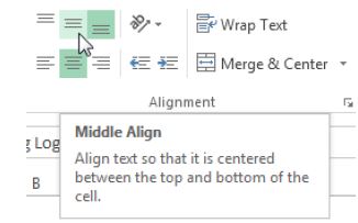
To change vertical text alignment
- Select the cell(s) you wish to modify.
- Select one of the three vertical alignment commands on the Home In our example, we'll choose Middle Align.
- The text will realign.
4.3. Cell borders and fill colors
Cell borders and fill colors allow you to create clear and defined boundaries for different sections of your worksheet.
To add a border
- Select the cell(s) you wish to modify.
- Click the drop-down arrow next to the Borders command on the Home The Borders drop-down menu will appear.

- Select the border style you want to use.
- The selected border style will appear.
- TIP: You can draw borders and change the line style and color of borders with the Draw Borders tools at the bottom of the Borders drop-down menu.

To add a fill color
- Select the cell(s) you wish to modify.
- Click the drop-down arrow next to the Fill Color command on the Home The Fill Color menu will appear.
- Select the fill color you want to use. A live preview of the new fill color will appear as you hover the mouse over different options. In our example, we'll choose Light Green.

- The selected fill color will appear in the selected cells.
4.4. Cell styles
Rather than formatting cells manually, you can use Excel's predesigned cell styles. Cell styles are a quick way to include professional formatting for different parts of your workbook, such as titles and headers.
To apply a cell style
- Select the cell(s) you wish to modify.
- Click the Cell Styles command on the Home tab, then choose the desired style from the drop-down menu.

- The selected cell style will appear.
- TIP: Applying a cell style will replace any existing cell formatting except for text alignment. You may not want to use cell styles if you've already added a lot of formatting to your workbook.
4.5. Formatting text and numbers
One of the most powerful tools in Excel is the ability to apply specific formatting for text and numbers. Instead of displaying all cell content in exactly the same way, you can use formatting to change the appearance of dates, times, decimals, percentages (%), currency ($), and much more.
To apply number formatting
- Select the cells(s) you wish to modify.
- Click the drop-down arrow next to the Number Format command on the Home The Number Formatting drop-down menu will appear.
- Select the desired formatting option.
- The selected cells will change to the new formatting style.
Challenge!
- Open an existing Excel 2013 workbook.
- Select a cell and change the font style, size, and color of the text.
- Apply bold, italics, or underline to a cell.
- Try changing the vertical and horizontal text alignment for some cells.
- Add a border to a cell range.
- Change the fill color of a cell range.
- Try changing the formatting of a number.