Formulas and Functions
One of the most powerful features in Excel is the ability to calculate numerical information using formulas.
6.1. Simple Formulas
Just like a calculator, Excel can add, subtract, multiply, and divide. In this lesson, we'll show you how to use cell references to create simple formulas.
Mathematical operators
Excel uses standard operators for formulas, such as a plus sign for addition (+), a minus sign for subtraction (-), an asterisk for multiplication (*), a forward slash for division (/), and a caret (^) for exponents.

All formulas in Excel must begin with an equals sign (=). This is because the cell contains, or is equal to, the formula and the value it calculates.
Understanding cell references
While you can create simple formulas in Excel manually (for example, =2+2 or =5*5), most of the time you will use cell addresses to create a formula. This is known as making a cell reference. Using cell references will ensure that your formulas are always accurate because you can change the value of referenced cells without having to rewrite the formula.

By combining a mathematical operator with cell references, you can create a variety of simple formulas in Excel. Formulas can also include a combination of cell references and numbers, as in the examples below:

To create a formula
- Select the cell that will contain the formula.
- Type the equals sign (=). Notice how it appears in both the cell and the formula bar.

- Type the cell address of the cell you wish to reference first in the formula: cell D1 in our example. A blue border will appear around the referenced cell.
- Type the mathematical operator you wish to use. In our example, we'll type the addition sign (+).
- Type the cell address of the cell you wish to reference second in the formula: cell D2 in our example. A red border will appear around the referenced cell.
- Press Enter on your keyboard. The formula will be calculated, and the value will be displayed in the cell.
- TIP: If the result of a formula is too large to be displayed in a cell, it may appear as poundsigns (#######) instead of a value. This means that the column is not wide enough to display the cell content. Simply increase the column width to show the cell content.
Modifying values with cell references
The true advantage of cell references is that they allow you to update data in your worksheet without having to rewrite formulas.
- TIP: Excel will not always tell you if your formula contains an error, so it's up to you to check all of your formulas.
To create a formula using the point-and-click method
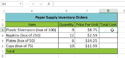
Rather than typing cell addresses manually, you can point and click on the cells you wish to include in your formula. This method can save a lot of time and effort when creating formulas. In our example below, we'll create a formula to calculate the cost of ordering several boxes of plastic silverware.
- Select the cell that will contain the formula. In our example, we'll select cell D3.
- Type the equals sign (=).
- Select the cell you wish to reference first in the formula: cell B3 in our example. The cell address will appear in the formula, and a dashed blue line will appear around the referenced cell.

- Type the mathematical operator you wish to use. In our example, we'll type the multiplication sign (*).
- Select the cell you wish to reference second in the formula: cell C3 in our example. The cell address will appear in the formula, and a dashed red line will appear around the referenced cell.

- Press Enter on your keyboard. The formula will be calculated, and the value will be displayed in the cell.

Formulas can also be copied to adjacent cells with the fill handle, which can save a lot of time and effort if you need to perform the same calculation multiple times in a worksheet.
To edit a formula
Sometimes you may want to modify an existing formula. In the example below, we've entered an incorrect cell address in our formula, so we'll need to correct it.
- Select the cell containing the formula you wish to edit.
- Click the formula bar to edit the formula. You can also double-click the cell to view and edit the formula directly within the cell.
- A border will appear around any referenced cells.
- When finished, press Enter on your keyboard or select the Enter command
 in the formula bar.
 - The formula will be updated, and the new value will be displayed in the cell.
- TIP: If you change your mind, you can press the Esc key on your keyboard or click the Cancel command
 in the formula bar to avoid accidentally making changes to your formula.
 - TIP: To show all of the formulas in a spreadsheet, you can hold the Ctrl key and press ` (grave accent). The grave accent key is usually located in the upper-left corner of the keyboard. You can press Ctrl+` again to switch back to the normal view.
Challenge!
- Open an existing Excel workbook.
- Create a simple addition formula using cell references.
- Try modifying the value of a cell referenced in a formula.
- Try using the point-and-click method to create a formula.
- Edit a formula using the formula bar.
6.2. Complex Formulas
A simple formula is a mathematical expression with one operator, such as 7+9. A complex formula has more than one mathematical operator, such as 5+2*8. When there is more than one operation in a formula, the order of operations tells Excel which operation to calculate first. In order to use Excel to calculate complex formulas, you will need to understand the order of operations.
Order of operations
Excel calculates formulas based on the following order of operations:
- Operations enclosed in parentheses
- Exponential calculations (3^2, for example)
- Multiplication and division, whichever comes first
- Addition and subtraction, whichever comes first
Creating complex formulas
In the example below, we will demonstrate how Excel solves a complex formula using the order of operations. Here, we want to calculate the cost of sales tax for an invoice. To do this, we'll write our formula as =(D2+D3)*0.075 in cell D4. This formula will add the prices of our items together and then multiply that value by the 7.5% tax rate (which is written as 0.075) to calculate the cost of sales tax.

- TIP: It is especially important to enter complex formulas with the correct order of operations. Otherwise, Excel will not calculate the results accurately. In our example, if the parentheses are not included, the multiplication is calculated first and the result is incorrect. Parentheses are the best way to define which calculations will be performed first in Excel.
Challenge!
- Open an existing Excel workbook.
- Create a complex formula that will perform addition before multiplication.
6.2.1. Relative and Absolute Cell References
There are two types of cell references: relative and absolute. Relative and absolute references behave differently when copied and filled to other cells. Relative references change when a formula is copied to another cell. Absolute references, on the other hand, remain constant, no matter where they are copied.
6.2.2. Relative cell references
By default, all cell references are relative references. When copied across multiple cells, they change basedon the relative position of rows and columns. For example, if you copy the formula =A1+B1 from row 1 to row 2, the formula will become =A2+B2. Relative references are especially convenient whenever you need to repeat the same calculation across multiple rows or columns.
To create and copy a formula using relative references
In the following example, we want to create a formula that will multiply each item's price by the quantity. Rather than creating a new formula for each row, we can create a single formula in cell D2 and then copy
it to the other rows. We'll use relative references so the formula correctly calculates the total for each item.
- Select the cell that will contain the formula. In our example, we'll select cell D2.
- Enter the formula to calculate the desired value. In our example, we'll type =B2*C2.

- Press Enter on your keyboard. The formula will be calculated, and the result will be displayed in the cell.
- Locate the fill handle in the lower-right corner of the desired cell. In our example, we'll locate the fill handle for cell D2.

- Click, hold, and drag the fill handle over the cells you wish to fill.

- Release the mouse. The formula will be copied to the selected cells with relative references, and the values will be calculated in each cell.
- TIP: You can double-click the filled cells to check their formulas for accuracy. The relative cell references should be different for each cell, depending on their rows.

6.2.3. Absolute cell references
There may be times when you do not want a cell reference to change when filling cells. Unlike relative references, absolute referencesdo not change when copied or filled. You can use an absolute reference to keep a row and/or column constant.
An absolute reference is designated in a formula by the addition of a dollar sign ($). It can precede the column reference, the row reference, or both.

You will generally use the $A$2 format when creating formulas that contain absolute references. The other two formats are used much less frequently.
- TIP: When writing a formula, you can press the F4 key on your keyboard to switch between relative and absolute cell references. This is an easy way to quickly insert an absolute reference.
To create and copy a formula using absolute references
In our example, we'll use the 7.5% sales tax rate in cell E1 to calculate the sales tax for all items in columnD. We'll need to use the absolute cell reference $E$1 in our formula. Since each formula is using the same tax rate, we want that reference to remain constant when the formula is copied and filled to other cells in column D.
- Select the cell that will contain the formula. In our example, we'll select cell D3.
- Enter the formula to calculate the desired value. In our example, we'll type =(B3*C3)*$E$1.
- Press Enter on your keyboard. The formula will calculate, and the result will display in the cell.

- Locate the fill handle in the lower-right corner of the desired cell.
- Release the mouse. The formula will be copied to the selected cells with an absolute reference, and the values will be calculated in each cell.
Challenge!
- Open an existing Excel workbook.
- Create a formula that uses a relative reference. Double-click a cell to see the copied formula and the relative cell references.
- Create a formula that uses an absolute reference.
6.3. Functions
A function is a predefined formula that performs calculations using specific values in a particular order. Excel includes many common functions that can be useful for quickly finding the sum, average, count, maximum value, and minimum value for a range of cells. In order to use functions correctly, you'll need to understand the different parts of a function and how to create arguments to calculate values and cell references.
Formula =A1+A2+A3+A4+A5+A6+A7+A8
Function =SUM(A1:A8)
The parts of a function
In order to work correctly, a function must be written a specific way, which is called the syntax. The basic syntax for a function is an equals sign (=), the function name (SUM, for example), and one or more arguments. Arguments contain the information you want to calculate.

Working with arguments
Arguments can refer to both individual cells and cell ranges and must be enclosed within parentheses. You can include one argument or multiple arguments, depending on the syntax required for the function.
For example, the function =AVERAGE(B1:B9) would calculate the average of the values in the cell range B1:B9. This function contains only one argument.

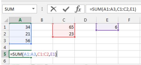
Multiple arguments must be separated by a comma. For example, the function =SUM(A1:A3, C1:C2, E2) will add the values of all the cells in the three arguments.
6.3.1. Creating a function
Excel has a variety of functions available. Here are some of the most common functions you'll use:
- SUM: This function adds all of the values of the cells in the argument.
- AVERAGE: This function determines the average of the values included in the argument. It calculates the sum of the cells and then divides that value by the number of cells in the argument.
- COUNT: This function counts the number of cells with numerical data in the argument. This function is useful for quickly counting items in a cell range.
- MAX: This function determines the highest cell value included in the argument.
- MIN: This function determines the lowest cell value included in the argument.
To create a basic function
In our example below, we'll create a basic function to calculate the average price per unit for a list of recently ordered items using the AVERAGE function.
- Select the cell that will contain the function.
- Type the equals sign (=) and enter the desired function name. You can also select the desired function from the list of suggested functions that will appear below the cell as you type. In our example, we'll type =AVERAGE.

- Enter the cell range for the argument inside parentheses. In our example, we'll type (D3:D12).
- Press Enter on your keyboard. The function will be calculated, and the result will appear in the cell.
To create a function using the AutoSum command
The AutoSum command allows you to automatically insert the most common functions into your formula, including SUM, AVERAGE, COUNT, MIN, and MAX. In our example below, we'll create a function to calculate the total cost for a list of recently ordered items using the SUM function.
- Select the cell that will contain the function.
- In the Editing group on the Home tab, locate and select the arrow next to the AutoSum command and then choose the desired function from the drop-down menu. In our example, we'll select Sum.

- The selected function will appear in the cell. If logically placed, the AutoSum command will automatically select a cell range for the argument. You can also manually enter the desired cell range into the argument.

- Press Enter on your keyboard.
6.3.2. The Function Library
While there are hundreds of functions in Excel, the ones you use most frequently will depend on the type of data your workbooks contains. There is no need to learn every single function, but exploring some of the different types of functions will be helpful as you create new projects. You can search for functions by category, such as Financial, Logical, Text, Date & Time, and more from the Function Library on the Formulas tab.
- To access the Function Library, select the Formulas tab on the Ribbon. The Function Library will appear.


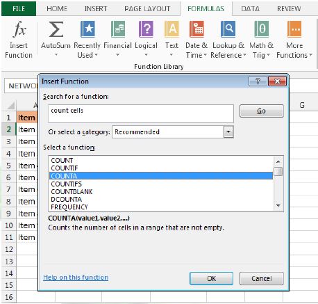
- If you're having trouble finding the right function, the Insert Function command allows you to search for functions using keywords.
- The AutoSum command allows you to automatically return results for common functions, like SUM, AVERAGE, and COUNT.
- The Recently Used command gives you access to functions that you have recently worked with.
- The Financial category contains functions for financial calculations like determining a payment (PMT) or interest rate for a loan (RATE).
- Functions in the Logical category check arguments for a value or condition. For example, if an order is over $50 add $4.99 for shipping, but if it is over $100, do not charge for shipping (IF).
- The Text category contains functions that work with the text in arguments to perform tasks, such as converting text to lowercase (LOWER) or replacing text (REPLACE).
- The Date & Time category contains functions for working with dates and time and will return results like the current date and time (NOW) or the seconds (SECOND).
- The Lookup & Reference category contains functions that will return results for finding and referencing information. For example, you can add a hyperlink (HYPERLINK) to a cell or return the value of a particular row and column intersection (INDEX).
- The Math & Trig category includes functions for numerical arguments. For example, you can round values (ROUND), find the value of Pi (PI) multiply (PRODUCT), subtotal (SUBTOTAL), and much more.
- More Functions contains additional functions under categories for Statistical, Engineering, Cube, Information, and Compatibility.
To insert a function from the Function Library
- Select the cell that will contain the function.
- Click the Formulas tab on the Ribbon to access the Function Library.
- From the Function Library group, select the desired function category.
- Select the desired function from the drop-down menu.

- The Function Arguments dialog box will appear. From here, you'll be able to enter or select the cells that will make up the arguments in the function.

- When you're satisfied with the arguments, click OK.
- The function will be calculated, and the result will appear in the cell.
Like formulas, functions can be copied to adjacent cells. Hover the mouse over the cell that contains the function, then click, hold, and drag the fill handle over the cells you wish to fill. The function will be copied, and values for those cells will be calculated relative to their rows or columns.

6.3.3. The Insert Function command
If you're having trouble finding the right function, the Insert Function command allows you to search for functions using keywords. While it can be extremely useful, this command is sometimes a little difficult to use. If you don't have much experience with functions, you may have more success browsing the Function Library instead. For more advanced users, however, the Insert Function command can be a powerful way to find a function quickly.
To use the Insert Function command
- Select the cell that will contain the function.
- Click the Formulas tab on the Ribbon, then select the Insert Function
- The Insert Function dialog box will appear.
- Type a few keywords describing the calculation you want the function to perform, then click Go.
- Review the results to find the desired function, then click OK.
- The Function Arguments dialog box will appear.
- When you're satisfied, click OK.
- The function will be calculated, and the result will appear in the cell.
Challenge!
- Open an existing Excel workbook.
- Create a function that contains one argument. If you're using the example, use the SUM function in cell B16 to calculate the total quantity of items ordered.
- Use the AutoSum command to insert a function.
- Explore the Function Library, and try using the Insert Function command to search for different types of functions.
Excel Formulas You Should Definitely Know
- SUM
Formula: =SUM(5, 5) or =SUM(A1, B1) or =SUM(A1:B5)
The SUM formula does exactly what you would expect. It allows you to add 2 or more numbers together.
You can use cell references as well in this formula.
- COUNT
Formula: =COUNT(A1:A10)
The count formula counts the number of cells in a range that have numbers in them.

It only counts the cells where there are numbers.
- COUNTA
Formula: =COUNTA(A1:A10)
Counts the number of non-empty cells in a range. It will count cells that have numbers and/or any other characters in them.
The COUNTA Formula works with all data types.

It counts the number of non-empty cells no matter the data type.
- LEN
Formula: =LEN(A1)
The LEN formula counts the number of characters in a cell. This includes spaces!

Notice the difference in the formula results: 10 characters without spaces in between the words, 12 with spaces between the words.
- VLOOKUP
Formula: =VLOOKUP(lookup_value, table_array, col_index_num, range_lookup)
Basically, VLOOKUP lets you search for specific information in your spreadsheet. For example, if you have a list of products with prices, you could search for the price of a specific item.
We’re going to use VLOOKUP to find the price of the Photo frame. You can probably already see that the price is $9.99, but that’s because this is a simple example. Once you learn how to use VLOOKUP, you’ll be able to use it with larger, more complex spreadsheets, and that’s when it will become truly useful.

As with any formula, you’ll start with an equal sign (=). Then, type the formula name.
=VLOOKUP(“Photo frame”
The second argument is the cell range that contains the data. In this example, our data is in A2:B16. As with any function, you’ll need to use a comma to separate each argument:
=VLOOKUP(“Photo frame”, A2:B16
Note: It’s important to know that VLOOKUP will always search the first column in this range. In this example, it will search column A for “Photo frame”. In some cases, you may need to move the columns around so that the first column contains the correct data.
The third argument is the column index number. It’s simpler than it sounds: The first column in the range is 1, the second column is 2, etc. In this case, we are trying to find the price of the item, and the prices are contained in the second column. That means our third argument will be 2:
=VLOOKUP(“Photo frame”, A2:B16, 2
The fourth argument tells VLOOKUP whether to look for approximate matches, and it can be either TRUE or FALSE. If it is TRUE, it will look for approximate matches. Generally, this is only useful if the first column has numerical values that have been sorted. Since we’re only looking for exact matches, the fourth argument should be FALSE. This is our last argument, so go ahead and close the parentheses:
=VLOOKUP(“Photo frame”, A2:B16, 2, FALSE)
And that’s it! When you press enter, it should give you the answer, which is 9.99.

- IF Statements
Formula: =IF(logical_statement, return this if logical statement is true, return this if logical statement is false).
Example
Let’s say a salesperson has a quota to meet. You used VLOOKUP to put the revenue next to the name. Now you can use an IF statement that says: “IF the salesperson met their quota, say “Met quota”, if not say “Did not meet quota”
=IF(C3>D3, “Met Quota”, “Did Not Meet Quota”)
This IF statement will tell us if the first salesperson met their quota or not. We would then copy and paste this formula along all the entries in the list. It would change for each sales person.
